Alfred Weber’s Theory of Industrial Location

Who was Alfred Weber?

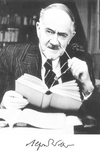
In this article, we will study Alfred Weber’s theory of industrial location. Alfred Weber was a German economist, geographer, sociologist and cultural philosopher. He was the younger brother of famous sociologist Max Weber. Born on July 30, 1868, in Erfurt and died on May 2, 1958, in Heidelberg, Weber started his carrier as a Lawyer and worked as a sociologist and cultural philosopher. Though his theory on ‘Industrial Location’ was strictly economic during his time it is widely studied in the field of geography now, mostly as a theoretical concept in the subdomain of economic geography, hence recognising Weber as an ‘Economic Geographer’ in the respective field, a discipline more contemporary. Alfred Weber is also known for the Weber Problem, a geometric median that aims to find out the minimum transport cost of a particular location.

Why a model or a theory?

A theoretical model in social sciences is a simplified version of real-life complexity. It may or may not be applicable directly but gives an overview of the situation. Such models are known as normative models i.e. models behind decision-making.

Such models answer an important, Where should we locate an industry?. Based on certain assumptions they help find the most optimal location for an industry. If we can narrow down on a location we can further try to make alterations and improvements in the real world.

Why a location theory in geography?

All the products produced today are complex with commodity supply chains spread across the geography. They go through different stages of production and consume multiple resources before transforming into the final product. An economic geographer tries to link the spatial geometry and proposes a median point to locate with maximum advantage.

Approaches to the problem of location

There are two approaches to understanding the problem of location

• Why some areas are attracted to industries? 
• Why some industries are attracted by certain areas? 

The first approach is a regional approach that tries to determine the advantages a particular region offers. The second try to isolate all the factors that affect the cost of production and examine them in relation to their location.

Factors that affect the location of an industry

They can be divided into two broad categories

• Geographical factors like land, climate, raw material, water, power, minerals, etc.
• Socio-economic factors

Capital, labour, transport, demand, market, government patronage and policies, tax structure, management, etc.

Location theories

The first theory that revolutionised the concept of industrial location was given by Alfred Weber in 1909. Published in the book ‘Uber den Standort der Industrien’ which translates to ‘The Location and Theory of Industries’ in English.

Alfred Weber’s least cost theory of locational analysis (or Alfred Weber’s Theory of Industrial Location), was based on suggestions made by Wilhelm Launhardt (German mathematician and economist) and became a very important subject in the fields of economic geography, regional science and spatial economics. The theories that followed Weber’s work were as follows…

• Alfred Weber’s Theory (1909)
• The theory of  Tard Padandnr (1935)
• The theory of Edgar Hoover (1937)
• The theory of Agust Losch (1954)
• The theory of Melvin Grceuhut (1956)
• The theory of Waiter Hard (1956)
• The theory of Fetter

---

The objective of the theory is…

“To find out minimum cost location of an Industry”

---

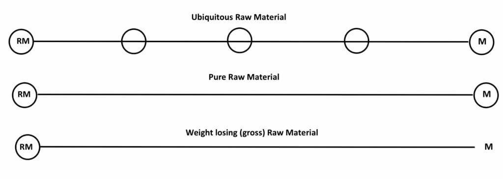
The terminology used in the theory

• Ubiquities– Materials available everywhere at the same cost (air, water)
• Localised Raw Materials – Materials available only at specific locations
• Pure Materials – Materials that enter to the full extent of their use  (RM=FP)
• Weight – losing (Gross Materials)– only a portion of their weight is transformed into finished products (RM>FP)
• Isotim – line of equal transport cost of any material or product
• Isodapane – lines connecting points of equal total transport cost

• Material Index(MI)   =    wt. Localised Raw Material (LRM)  / wt. Finished Product (FP)

a)  RM is more than FP;   MI>1

b)  RM is less than FP;      MI<1

c)  RM is equal to FP;        MI=1

Assumptions

Alfred Weber’s Theory of Industrial Location had the following assumptions

• Uniform or isotropic plain in a single country i.e. the geographical area considered.
• Labour is fixed geographically but its availability is unlimited.
• The raw materials are fixed at certain locations (known) and the point of consumption is also fixed and known. 
• Transportation costs are a direct function of the weight of item and the distance shipped.
• Perfect competition i.e. same product, same quality, same price. Also, there are enough buyers and sellers in the country. Hence demand and supply or quality have no effect on the decision-making process.
• Entrepreneurs are economic rationale, meaning he has full knowledge of the present technology available in their field and will try to minimize cost accordingly. Such an idol person is known as an ‘economic man‘.

The question one should ask here is…

Are these assumptions found in the real world? We should remember that Weber simplified a complex world and in order to see things simply certain things have to be hypothesised while holding some constant, only then the most important variables (location here) could be found out.

---

Role of Transport Cost

Transport is the most important factor in Weber’s theory and is a result of the total distance of haulage and the weight of material transported.

There are two conditions to study transport costs

• Transport costs with a single market and one source of raw material
• Transport cost with a single market and two sources of raw material (the classic locational triangle)

First Condition: One Market, One Raw material

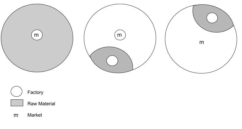
In Figure 1 (A) raw material is ubiquitous, factory locates at the market (point of lowest transport cost), as transporting a ubiquitous material will increase the cost.

In 1 (B) raw material is fixed, with no weight loss (pure), which means MI=1

factory locates at either market or raw material site.

In 1 (C) raw material is fixed with considerable weight loss (gross), MI>1

factory locates at the site of raw material. 

(In case of MI<1, i.e. Raw material is more than the finished product, the factory might again locate near the market)

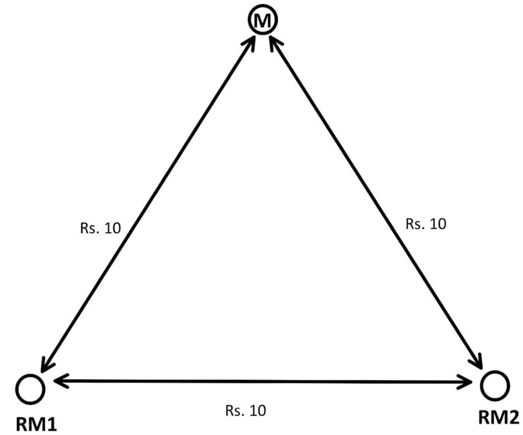
Second Condition: One Market, Two Raw Materials

Case 1

Two Pure Raw Materials

Again as shown in Figure (2) 

the shortest distance to the market is directly from point RM to M and will incur Rs. 20 transport cost. 

Any intermediary location will be a diversion from the shortest route and will incur an unnecessary logistic cost.

Case 2

Two Weight-Losing Raw Materials

In Figure (3) raw material is weight losing and weight loss will pull the industry close to the source of raw material RM1, RM2 and away from the market.

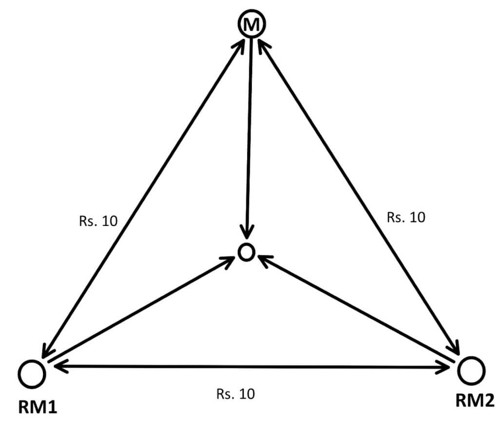
1. How did we conclude that in Case 2 the best location will be somewhere in between the triangle?
2. Where exactly ‘in between’ is?

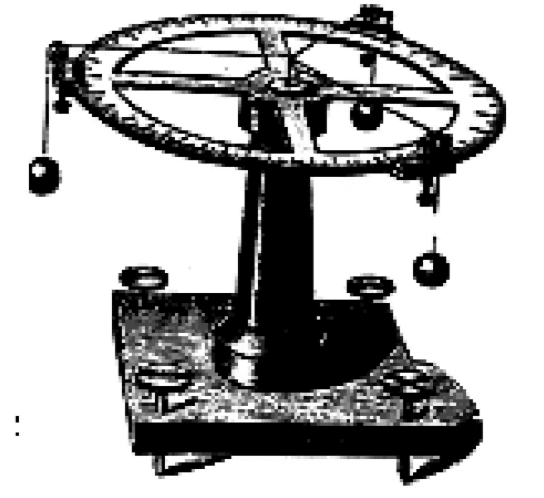
To answer these questions as suggested by Weber, we have to take the help of the Varignon Frame (Fig. 4).

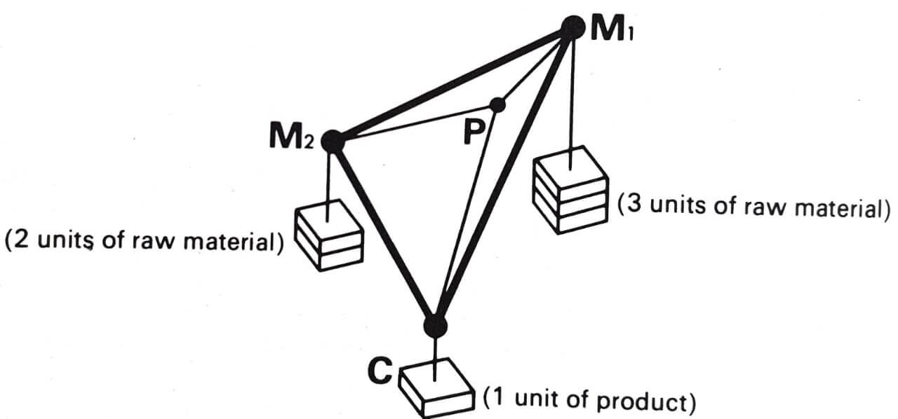
It is a hardware model with strings and pulleys on a wooden frame (Fig. 4 & 5). Each string has some weights attached to it. The heavier the weight, the more the force in that direction and the more it pulls the knot P towards itself. Knot P is the optimal location for the industry. Heavier weights pull the industry towards itself.

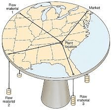
If the material is weight-losing it will have a heavier proportion of weight on the pullies and a percentage of that weight will not add to the final weight of the product. This means more weight loss will exert more pull and pull the industry in its direction.

---

Split of Location

---

Role of labour cost

Spatial distribution of transport cost

• As transport costs lay at the heart of this model Weber devised a technique to measure and map the spatial differences in these costs
• To find the LCL (lowest cost location)
• He produced two types of contour lines
  • Isotims
  • Isodapanes

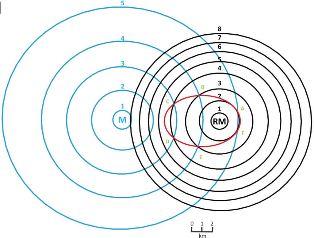
In fig. 6, M represents the market and RM represents the raw material. Concentric circles around it are countors or iso-lines representing transport costs as one moves away from the market and raw material.

According to figure 6

M – Market

(blue circles are far, therefore…)

• The cost of transporting the finished product is Rs. 0.5 for 1 km
• numbers 1-5 written on blue lines represent Rs. spent on the transportation of the finished product.

RM – Raw Material Source

(black circles are close, therefore…)

• Cost of transporting raw material Rs. 1 for 1 km
• numbers 1-8 written on black lines represent Rs. spent on the transportation of raw material.

Isotims

These blue and black lines are known as isotims and they represent transport costs for both finished products from the market (blue lines) with greater counter interval and transport cost from the source of raw material (lesser counter interval). The material with close contour interval i.e. steep increment will be more expensive to transport as its cost changes rapidly (raw material in this case).

Isodapanes

We can see that in fig. 6 blue and black isotim lines of M and RM intersect at many points. But it is only at A, B, C, D, E & F the cost of transportation is minimum. 

A_ 2+5=7, B_3+4=7, C_4+3=7, D_3+4=7, E_4+3=7, F_5+2=7

Isodapanes are the lines connecting places of equal transport cost. Here this cost is Rs. 7. 

There can be multiple isodapanes. As shown in Figure 7.

---

Weber gave the following formula to measure the attracting power of labour

Labour Coefficient =   Labour Cost Index / Locational Weight

It is measured by labour cost index i.e. proportion of labour cost to the weight of the finished product 

The higher the labour coefficient, the greater is the tendency for a plant to be located near the centre of cheap labour supply.

Effect of Cheap Labour

Critical Isodapane

The creation of the concept of *critical isodapane – the set of points that equals the rise in transport costs to smaller wage costs. Changes in the industry location happen if the point of cheaper labour cost is within the critical isodapane

where savings in labour cost are > than the added costs of transport incurred when moving closer to the  cheaper labour supply

Lead by a labour coefficient  the higher the index, the greater the likelihood of the industry’s diversion from the LCL

*Critical Isodapane is the point where Transportation Cost = Labour Cost. Where both labour cost and transport cost are minimum as compared to their total cost anywhere else. Isodapanes drawn to the point beyond which there is no labour advantage (Figure 7).

---

Agglomeration of Economies

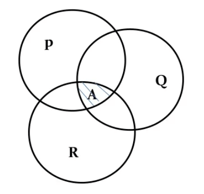
The region between three intercepting isodapanes is Agglomeration, referring to the clustering of industrial plants to achieve LCL through:

• the reduction of inter-factory transport costs
• greater specialization
• the use of larger machinery
• an established pool of skilled labour and expertise
• the prestige/reputation
• the development of local market knowledge.

*It uses the same ratio as the labour coefficient.

---

Limitations of the theory

Alfred Weber’s Theory of Industrial Location was much ahead of its time but certainly, it had the following shortcomings

• Modes of transport competition between different transport systems, freight rates rarely directly proportional to the distance
• Rigid assumption of the isotropic surface.
• Prices factors of production and market prices were not fixed
• Government intervention in the location of industries has grown eg zoning laws, subsidies, taxes, etc
• Weight loss assumptions are narrow for value-added products. Other qualities of raw materials also have an impact on industrial location
• Immobile labour

---

949 views