
Digital image processing refers to using algorithms and computer systems to manipulate and analyse digital images. Satellite and aerial sensors capture vast amounts of data about the Earth’s surface, by processing this data, researchers and professionals can extract valuable information for various applications, such as environmental monitoring, urban planning, agriculture, and natural resource management.
Digital image processing involves multiple steps, from pre-processing raw data to enhance its quality, to complex transformations and classifications that provide actionable insights. This page outlines these steps in a structured manner.
Pre-Processing
Pre-processing is the initial step in digital image processing that focuses on improving the quality of raw data captured by sensors. Remote sensing data often contains distortions and inconsistencies caused by various factors, such as atmospheric interference, sensor errors, or geometric distortions. Pre-processing aims to correct these issues and prepare the data for further analysis. Key components of pre-processing include:
Radiometric Correction
When satellites, aircraft, or drones capture images of the Earth’s surface using remote sensing technologies, the data they collect is not a direct, unaltered reflection of the physical properties of the terrain. Instead, the observed electromagnetic energy is influenced by many factors that occur between the sensor and the target area. These factors include the sun’s position and angle relative to both the sensor and the Earth’s surface, the variable atmospheric conditions such as cloud cover, humidity, and the presence of aerosols, and the inherent characteristics and performance of the sensor itself.
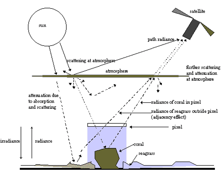
The sun’s position affects how bright and from which angle light hits the ground, causing changes in reflected light that aren’t just from the ground’s materials or texture. Atmospheric conditions can further distort the signal by scattering and absorbing certain wavelengths of light, introducing a form of “noise” into the data that obscures the true signals from the Earth’s surface. Additionally, sensors are not perfectly uniform in their response; they can exhibit variations in sensitivity across different parts of their field of view or over time due to degradation and other operational factors. These radiometric distortions complicate the interpretation and analysis of remotely sensed data. To derive meaningful information about the Earth’s surface, such as land cover types, vegetation health, surface temperatures, or mineral compositions, it is essential to correct these effects.
Radiometric correction is the process of applying mathematical and statistical techniques to the raw data to mitigate the impacts of these distortions, thereby improving the accuracy and reliability of the information extracted from the images. The primary objective of radiometric correction is to enhance the fidelity of the brightness values represented in the digital images, ensuring that these values more closely correspond to the actual radiance or reflectance properties of the Earth’s surface features. By doing so, radiometric correction enables more accurate and consistent comparisons of data collected at different times, from different sensors, or under varying environmental conditions.
| Step | Description |
|---|---|
| Detector Response Calibration | Ensures uniform response of all detectors in a sensor array by correcting inconsistencies caused by ageing, manufacturing defects, or environmental conditions. Corrects striping or banding artefacts in the image. |
| Sun Angle and Topographic Correction | Accounts for illumination variations due to sun angle and surface topography, standardizing pixel values for consistent reflectance measurements. |
| Atmospheric Correction | Ensures uniform response of all detectors in a sensor array by correcting inconsistencies caused by aging, manufacturing defects, or environmental conditions. Corrects striping or banding artefacts in the image. |
Detector Response Calibration
In remote sensing, “detector response calibration” refers to the process of standardizing the signals recorded by multiple detectors within a sensor to ensure uniform and accurate data across the entire image. Sensors often use an array of detectors, each of which may respond differently to the same incoming radiation due to slight manufacturing imperfections, ageing, or operational conditions. These variations can cause visible artefacts, such as “striping” (alternating bright and dark lines) or other inconsistencies in the imagery.
Detector response calibration addresses these discrepancies by adjusting each detector’s output to match a consistent baseline. This is typically achieved through a combination of methods, including:
- Pre-launch calibration: Laboratory testing and adjustment of detectors before the sensor is deployed.
- On-orbit calibration: Using known reference targets, such as uniform Earth features or onboard calibration sources, to monitor and correct for changes in detector performance over time.
- Post-processing techniques: Algorithms are applied to correct issues like striping, missing scan lines, random noise, and vignetting in the collected imagery.
Main components of detector response calibration
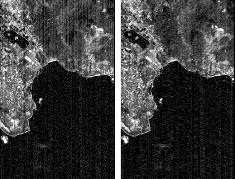
De-striping
This process addresses the issue of striping artefacts that often appear in satellite images. Inconsistencies in the response of different detectors within the sensor cause these stripes. De-striping algorithms analyze the image data to identify and correct these variations, resulting in a more uniform and visually appealing image. Technically, de-striping involves analyzing the statistical or frequency characteristics of the image to isolate the stripe pattern from the actual signal. Key methods for de-striping include:
- Mathematical Basis of De-striping: To address stripe artefacts, de-striping algorithms often model the detected signal as a combination of the true signal and stripe noise.$$\text{Mathematically, for a pixel \((x, y)\)} \\ \text{in an image:}\\ \begin{equation} I(x, y) = S(x, y) + N_{\text{stripe}}(x, y) \end{equation}\\ \text{Where:}\\ \text{ – } I(x, y) \text{ represents the observed intensity at pixel } (x, y),\\ \text{ – } S(x, y) \text{ is the true signal,}\\ \text{ – } N_{\text{stripe}}(x, y) \text{ denotes the stripe noise,}\\ \text{ – } N_{\text{stripe}}(x, y) \text{ is typically modelled as a spatially or } \\ \text{ temporally periodic variation introduced by detector inconsistencies.}$$
- Simplified Explanation: Mathematically, for each pixel (x, y)in an image: We have an equation that says: $$ I(x, y) = S(x, y) + N_{\text{stripe}}(x, y) $$ What does this mean? I(x, y) This is the brightness or intensity of the pixel at position (x, y) that we see in the image. – S(x, y) This is the actual, true brightness or signal that the object at that pixel should have, without any noise. – $$N_{\text{stripe}}(x, y)$$ This represents the “stripe noise” — an unwanted pattern that appears as stripes in the image. This noise is usually caused by small differences in how different parts of the camera or detector work. The stripe noise $$N_{\text{stripe}}(x, y)$$ often happens in a regular, repeating pattern (spatially or temporally) because of slight inconsistencies in the detector or camera components that take the picture. So, the equation tells us that the observed intensity at each pixel I(x, y) is the sum of the true signal S(x, y) and the unwanted stripe noise $$N_{\text{stripe}}(x, y)$$ In simple terms: What we see in the picture (I) is the real thing (S) plus some annoying stripes $$(N_{\text{stripe}})$$
Common Techniques for Destriping
- Statistical Normalization: In this method, the mean and standard deviation of pixel values for each detector line (or column) are normalized to match a global or reference standard. $$\text{For a detector } d,\\ \text{ the normalized value } I_{\text{norm}}(x,y) \text{ is computed as:}\\ \begin{equation} I_{\text{norm}}(x,y) = \frac{I(x,y) – \mu_d}{\sigma_d} \cdot \sigma_{\text{ref}} + \mu_{\text{ref}} \end{equation}\\ \text{Where:}\\ \text{ – } \mu_d, \sigma_d \text{ : Mean and standard deviation for detector } d,\\ \text{ – } \mu_{\text{ref}}, \sigma_{\text{ref}} \text{ : Mean and standard deviation of the reference detector or entire image.}$$
- Fourier Transform-Based Filtering: Stripe artefacts often appear as high-energy components at specific frequencies in the Fourier domain. By applying a Fourier transform to the image: $$F(u,v) = \sum_{x=0}^{M-1} \sum_{y=0}^{N-1} I(x,y) \cdot e^{-j2\pi\left(\frac{ux}{M} + \frac{vy}{N}\right)}$$ Stripe noise frequencies are identified and suppressed by applying a notch filter or band-reject filter, leaving the true signal S(x,y)S(x, y)S(x,y) intact.
- Wavelet Transform: Wavelet transforms decompose the image into multiple frequency components, enabling stripe noise$$N_{\text{stripe}}(x,y)$$to be isolated at specific scales. The wavelet coefficients corresponding to stripe artefacts are suppressed before reconstructing the corrected image: $$I_{\text{corrected}}(x,y) = W^{-1}\{W(I(x,y)) – W(N_{\text{stripe}}(x,y))\}$$ $$\text{Where }\\ W \text{ and } W^{-1} \text{ represent the wavelet transform and its inverse.}$$
- Adaptive Filtering: Adaptive filtering involves applying spatial filters, such as median filters or high-pass filters, to detect and remove stripe patterns while maintaining the structural integrity of the image.
- Median Filter: This filter replaces the intensity of each pixel with the median value within a defined local window (e.g., 3×3 or 5×5). This process is highly effective at removing linear stripe artefacts because it suppresses outliers while preserving edges and fine details in the image. Mathematically, for a pixel I(x,y)I(x, y)I(x,y), the median filter output can be represented as: $$I_{\text{filtered}}(x,y) = \text{median}\{I(x+i,y+j) \mid (i,j) \in \text{window}\}$$ High-Pass Filter: This filter enhances high-frequency components by suppressing low-frequency regions. It can isolate and correct stripe patterns, which often manifest as low-frequency anomalies in the image.
- Adaptive filtering is particularly useful in removing stripe noise in images where noise patterns are predictable but require the preservation of spatial features.
- Principal Component Analysis (PCA): PCA is a statistical technique often employed to remove stripe noise by decomposing the image into its principal components. Stripe artefacts, being highly correlated in one direction, often dominate certain principal components and can be treated as noise. The steps involved in PCA-based de-striping are:
- Decomposition: The image data I is transformed into its principal components, typically through eigenvalue decomposition or singular value decomposition (SVD). Mathematically: $$ I = U\Sigma V^\top,\\ \text{ where:}\\ U \text{ and } V \text{ are orthogonal matrices,}\\ \Sigma \text{ is a diagonal matrix containing the singular values.} $$
- Noise Identification: Principal components associated with stripe noise are identified by their high variance or specific directional characteristics.
- Reconstruction: The noisy components are discarded, and the image is reconstructed using the remaining components:$$I_{\text{reconstructed}} = U’ \Sigma’ V’^\top. \\ \text{where } \\U’, \Sigma’, \text{ and } V’ \text{ exclude the noise-dominated components.}$$ PCA is particularly powerful in applications where stripe patterns dominate specific frequency bands or components, allowing for effective separation and removal of noise while preserving image details.
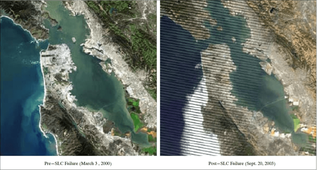
Removal of Missing Scan Line:
In remote sensing, line dropout occurs when a detector either fails temporarily or becomes saturated during the scanning process. This results in the loss of data along specific scan lines, creating horizontal streaks or gaps in the image. Addressing these issues is crucial to ensure the image remains useful for analysis. The process of correcting missing scan lines involves estimating the lost data using values from adjacent lines in the image.
- Single Missing Line Correction: When a single scan line is missing, its values are estimated by averaging the pixel values from the lines immediately above and below the missing line. This ensures a smooth transition without abrupt changes in pixel intensity. The formula for estimating the pixel value is: $$ \text{DN}_{x,y} = \frac{\text{DN}_{x,y-1} + \text{DN}_{x,y+1}}{2} \text{Where:}\\ \text{DN}_{x,y} \text{ : Pixel value in the missing line at position } x,y.\\ \text{DN}_{x,y-1} \text{ : Pixel value in the line above the missing line.}\\ \text{DN}_{x,y+1} \text{ : Pixel value in the line below the missing line.}$$
- Two Consecutive Missing Line: If two consecutive lines are missing:
- The first missing line is replaced by duplicating the values of the previous line.
- The second missing line is replaced by duplicating the values of the subsequent line.
- This approach ensures continuity but does not introduce interpolation errors.
- Three Consecutive Missing Lines: For three consecutive missing lines:
- The first line is replaced by repeating the previous line.
- The third line is replaced by repeating the subsequent line.
- The middle line is interpolated by averaging the pixel values of the first and third lines:$$ \text{DN}_{x,y} = \frac{\text{DN}_{x,y-1} + \text{DN}_{x,y+3}}{2} $$
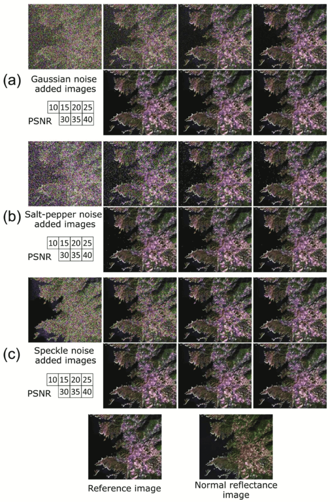
Random Noise Removal
Random noise is a significant challenge in remote sensing imagery, characterized by irregular and unpredictable variations in pixel values. It degrades image quality, reducing the reliability of data for analysis. Random noise can originate from several sources, such as sensor electronics, atmospheric interference, and environmental factors during image acquisition. Proper random noise removal enhances image clarity, enabling more precise interpretation and analysis for remote sensing applications.
Types of Random Noise
Random noise in remote sensing can take on various forms, each with unique characteristics and origins. Understanding these types is crucial for selecting appropriate techniques to mitigate their effects and improve the quality of the imagery. Below are the most common types of random noise encountered in remote sensing data:
- Gaussian Noise also known as normal noise, is characterised by pixel intensity values that follow a normal distribution. This means the noise is distributed symmetrically around a mean value, typically zero. The majority of variations are small, while extreme deviations are rare. Gaussian noise often originates from electronic components in sensors, such as thermal noise or voltage fluctuations, which are inherent in the data acquisition process.
- Salt-and-pepper noise appears as randomly scattered bright (salt) and dark (pepper) pixels throughout the image. This type of noise is typically caused by abrupt disruptions in data transmission, sensor malfunctions, or digital errors during recording. This noise creates a speckled, irregular appearance that can mask fine details, making it challenging to interpret specific features.
- Speckle noise is unique to coherent imaging systems, such as radar and synthetic aperture radar (SAR). It arises due to the interference of coherent electromagnetic waves reflected from multiple scatterers within a single pixel. These scatterers, such as vegetation or rough surfaces, create a granular pattern of noise across the image. Speckle noise reduces the contrast of radar images and can obscure surface patterns, such as water flow directions or geological structures.
- Periodic noise (Less common) is a rarer type of random noise that manifests as repetitive patterns, such as waves or lines, in the imagery. It is often caused by mechanical or electrical interference during data acquisition. These repetitive patterns can distort large portions of the image and interfere with edge detection or pattern recognition.
| Noise Type | Appearance | Source | Impact on Image |
|---|---|---|---|
| Gaussian Noise | Grainy texture | Sensor electronics, thermal noise | Alters pixel values subtly, reducing feature clarity |
| Salt-and-Pepper | Bright and dark pixel outliers | Sensor malfunctions, data transmission errors | Disrupts fine details, creates highly visible artifacts |
| Speckle Noise | Granular texture | Coherent wave interference (e.g., radar) | Reduces contrast, obscures surface patterns |
| Periodic Noise | Repetitive patterns (waves/lines) | Mechanical/electrical interference | Creates large-scale artifacts, distorting analysis |
- Techniques for Random Noise Removal: Various filtering techniques are used to mitigate random noise in remote sensing images. These methods aim to smooth the noisy areas while preserving important features, such as edges and fine details. Below are commonly used techniques:
- Median Filtering: A median filter replaces the value of a pixel with the median value of its surrounding pixels within a local window. It is highly effective at removing salt-and-pepper noise while preserving edge details. For a window size of 3×33 \times 33×3, the formula is: $$ \text{DN}_{x,y} = \text{Median}\{\text{DN}_{i,j} \mid (i,j) \in W_{x,y}\} \\ \text{Where } \\W_{x,y} \text{ is the set of pixels in the local window around pixel } (x,y)$$
- Low-Pass Filtering: A low-pass filter smooths the image by averaging the pixel values in a local window. While effective at reducing noise, it may blur fine details and edges. A simple low-pass filter applies the following operation: $$ \text{DN}_{x,y} = \frac{1}{n} \sum_{(i,j) \in W_{x,y}} \text{DN}_{i,j} \\ \text{Where } \\n \text{ is the number of pixels in the window.}$$
- Adaptive Filtering: Adaptive filters consider both the local mean and variance to distinguish between noise and true features in the image. These filters are particularly useful in heterogeneous areas, as they preserve edges and details better than simple low-pass filters. A common adaptive filter formula is: $$ \text{DN}_{x,y} = \text{DN}_{x,y} + k \cdot (\text{DN}_{\text{local mean}} – \text{DN}_{x,y}) \\\text{Where } \\k \text{ is an adaptation coefficient based on local variance.}$$
- Gaussian Filter: A Gaussian filter minimizes abrupt changes in pixel intensity by applying a Gaussian kernel, which smooths the image and reduces Gaussian noise. In 2D convolution, it is widely used in remote sensing to suppress random noise while slightly blurring the image.
- Mean Filter: This linear filter replaces each pixel’s intensity with the mean value of its neighbours in a defined window. It effectively reduces overall noise levels but may blur sharp edges or fine details.
- Standard Median Filter: A non-linear filter that replaces each pixel’s intensity with the median value in its neighbourhood. It is particularly effective at removing salt-and-pepper noise without significantly blurring edges, but its performance can degrade with asymmetrical noise distributions.
- Adaptive Median Filter: An enhancement of the standard median filter, this method dynamically adjusts the window size for each pixel based on local noise levels. It is ideal for preserving fine details in areas with varying noise intensities.
- Adaptive Wiener Filter: This filter adapts to local statistical properties, such as mean and variance, within the filter window. While it is computationally more intensive, it excels at removing Gaussian noise while preserving edges and textures, making it highly effective for remote sensing data.
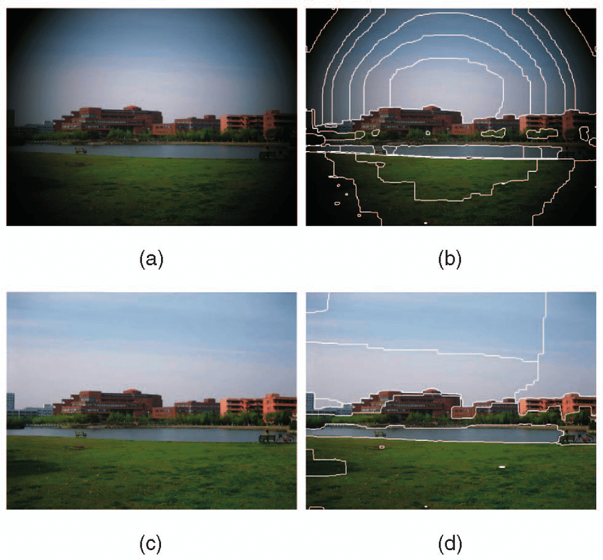
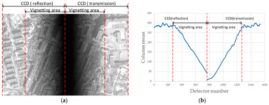
Vignetting Removal
Vignetting refers to the gradual reduction of brightness or intensity at the edges of an image compared to its centre. This phenomenon is a common issue in remote sensing and occurs due to imaging systems’ optical and mechanical limitations. It introduces non-uniformity in the captured imagery, which can affect the accuracy of subsequent analysis, especially in quantitative remote sensing applications like vegetation indices or land cover classification.
Vignetting introduces bias in pixel intensity values, reducing radiometric accuracy. It also affects the reliability of quantitative data extraction, such as reflectance values. Due to brightness inconsistencies, it impacts visual interpretation and object identification.
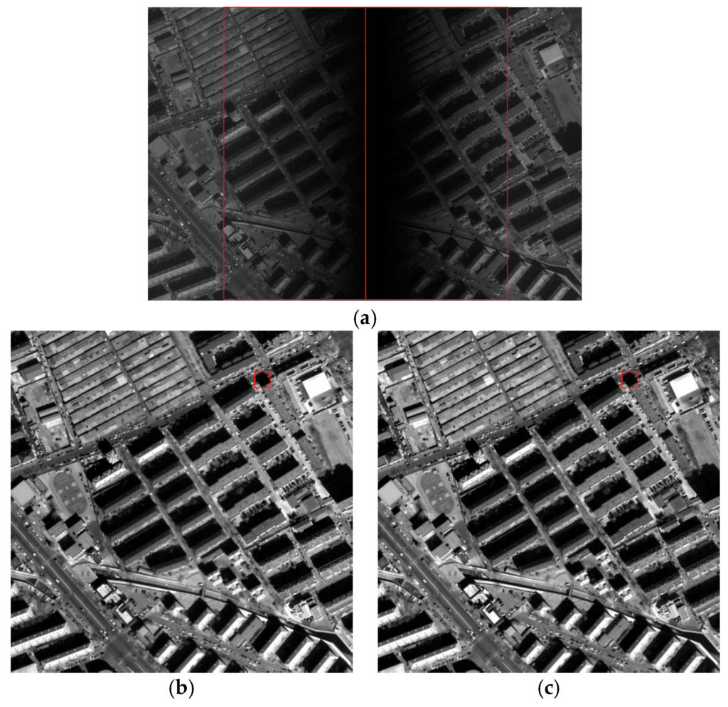
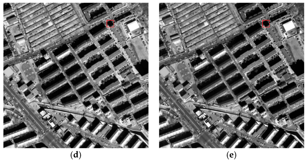
- Methods for Vignetting Removal: Vignetting removal aims to correct the non-uniform illumination across the image, ensuring that the pixel values are consistent and accurately represent the observed surface. The main methods include:
- Flat-Field Correction: This method involves dividing the original image by a reference image captured under uniform illumination, known as a flat-field image. $$ I_{\text{corrected}}(x,y) = \frac{I_{\text{flat}}(x,y)}{I_{\text{observed}}(x,y)} \cdot I_{\text{mean}} \\ \text{where } \\I_{\text{observed}} \text{ is the original image, }\\ I_{\text{flat}} \text{ is the flat-field image,}\\ \text{and } I_{\text{mean}} \text{ is the mean intensity of the flat field to maintain brightness.}$$
- Polynomial fitting is a method used to correct vignetting by modelling the intensity variations in the image with a low-order polynomial. The brightness gradient caused by vignetting is analyzed, and a smooth polynomial surface is fitted to represent the intensity drop-off. This fitted surface serves as a correction model, and the pixel values in the image are adjusted by either subtracting or dividing them by the polynomial surface.
- Cosine Fourth Power Law Correction: Vignetting is often approximated using the cosine fourth power law, which accounts for light falloff as a function of the angle of incidence:$$ I_{\text{corrected}}(x,y) = I_{\text{observed}}(x,y) \cdot \cos^4(\theta) \\ \text{where }\\ \theta \text{ is the angle between the optical axis} \\ \text{and the light rays hitting the sensor.}$$
- Image Histogram Matching: Histogram matching, also known as histogram specification, is a technique in digital image processing used to adjust the intensity distribution of an image to match the histogram of a reference image. This method is often applied in remote sensing to achieve uniformity between images captured under different conditions or to enhance specific features for better interpretation and analysis.
- Software-Based Approaches: Modern image processing software (e.g., ENVI, ERDAS, QGIS) includes vignetting correction tools that apply automated algorithms, often combining flat-field correction and histogram equalisation techniques.
Sun Angle and Topographic Correction
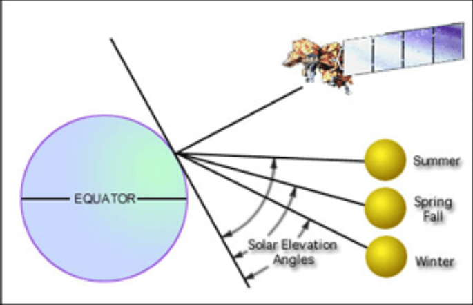
These corrections account for how the sun’s position and the Earth’s terrain influence the illumination and reflectance of surface features. Sun angle and topographic correction address the variations in pixel brightness caused by the uneven illumination of Earth’s surface due to changes in solar geometry (sun angle) and the topographic features of the terrain. Without this correction, surface reflectance values can be misinterpreted, especially in areas with significant terrain variability, such as mountainous regions.
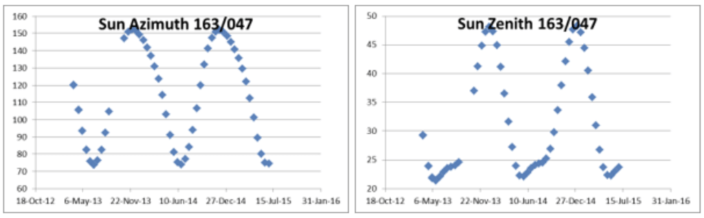
- Sun Angle Correction: The position of the sun changes throughout the day and year, affecting the amount of light that reaches the Earth’s surface. This variation influences the reflectance values captured by sensors.
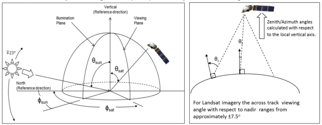
- Solar Zenith Angle: The angle between the sun’s rays and the vertical direction at a given location. Larger zenith angles reduce the intensity of direct solar radiation.
- Solar Azimuth Angle: The angle of the sun in the horizontal plane, affects the direction of illumination.
- Topographic Correction: The Earth’s surface is not flat, and terrain features like hills and valleys can cast shadows and alter the local illumination conditions. Topographic correction uses digital elevation models (DEMs) to simulate the effects of terrain on light distribution and adjusts the image data accordingly, providing a more accurate representation of surface reflectance.errain features such as slopes and aspects (the direction a slope faces) cause differential illumination.
- Sunlit Slopes: Slopes facing the sun receive more radiation, leading to higher reflectance.
- Shaded Slopes: Slopes facing away from the sun receive less radiation, leading to lower reflectance.
Sun Angle and Topographic Correction Methods
- Cosine Correction: This basic approach adjusts pixel values based on the cosine of the solar zenith angle: $$ R_{\text{corrected}} = \frac{R_{\text{observed}}}{\cos(\theta_s)} \\ \text{Where:}\\ R_{\text{observed}} \text{ : Observed reflectance.}\\ \theta_s \text{ : Solar zenith angle.}$$ While simple, cosine correction does not account for the effects of topography (e.g., slopes and aspects).
- C-Correction: A more advanced method that incorporates topographic information (e.g., slope and aspect): $$ R_{\text{corrected}} = R_{\text{observed}} \cdot \left( \frac{\cos(\theta_i) + c}{\cos(\theta_s) + c} \right) \\ \text{Where:}\\ \theta_i \text{ : Local incidence angle (angle between the sun’s rays and the surface normal).}\\ c \text{ : Empirical constant derived from regression analysis of observed reflectance and illumination angles.}$$The C-correction improves reflectance normalization by accounting for terrain-induced illumination variability.
- Minnaert Correction: This method models the relationship between illumination and reflectance as a power-law function: $$ R_{\text{corrected}} = R_{\text{observed}} \cdot \left( \frac{\cos(\theta_s)}{\cos(\theta_i)} \right)^k $$Where kkk is the Minnaert constant, determined empirically for the specific surface type. This method is effective in areas with heterogeneous terrain.
- Topographic Normalization Using DEM: A digital elevation model (DEM) provides slope and aspect information, allowing for more accurate correction:$$ \cos(\theta_i) = \cos(\theta_s) \cdot \cos(\beta) + \sin(\theta_s) \cdot \sin(\beta) \cdot \cos(\phi – \phi_s) \\ \text{Where:}\\ \beta \text{ : Slope angle.}\\ \phi \text{ : Aspect angle.}\\ \phi_s \text{ : Solar azimuth angle.}$$ This approach ensures that pixel reflectance values represent true surface conditions by compensating for both sun angle and terrain effects.
Atmospheric Correction
Atmospheric correction is a critical step in remote sensing to ensure the accuracy of satellite or aerial imagery. As electromagnetic radiation travels through the Earth’s atmosphere, it undergoes scattering, absorption, and reflection by atmospheric gases, aerosols, and particulates. These interactions can significantly alter the spectral and radiometric characteristics of the reflected radiation captured by sensors. Atmospheric correction techniques aim to mitigate these distortions, allowing accurate representation of surface reflectance, which is essential for quantitative remote sensing and reliable analysis.
Components of Atmospheric Effects
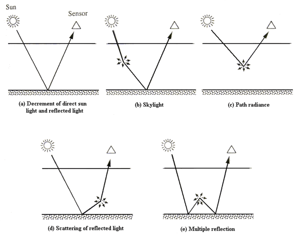
- Scattering
- Scattering occurs when atmospheric particles and gases disrupt the path of radiation. It is wavelength-dependent and categorized as:
- Rayleigh Scattering: Dominates in shorter wavelengths (e.g., blue region), caused by atmospheric molecules smaller than the wavelength.
- Mie Scattering: Occurs due to larger particles (e.g., dust, water droplets), impacting longer wavelengths.
- Non-Selective Scattering: Affects all wavelengths equally, caused by particles larger than the wavelength, such as cloud droplets.
- Scattering occurs when atmospheric particles and gases disrupt the path of radiation. It is wavelength-dependent and categorized as:
- Absorption
- Atmospheric gases, such as water vapor (H₂O), carbon dioxide (CO₂), and ozone (O₃), absorb radiation at specific wavelengths, leading to spectral distortions.
- Path Radiance
- The scattered light that directly enters the sensor without interacting with the Earth’s surface contributes to path radiance. This increases the brightness of the image and alters spectral characteristics.
Methods of Atmospheric Correction
Atmospheric correction methods can be broadly classified into two categories: empirical methods and physical or model-based methods.
Empirical Methods
- Dark Object Subtraction (DOS)
- This method assumes that some areas in the image, such as deep water bodies or shadows, have near-zero reflectance. The observed radiance from these areas is attributed to atmospheric effects and subtracted from the entire image.
- Steps:
- Identify pixels with low reflectance in all bands (dark objects).
- Subtract their radiance values from the image to eliminate atmospheric effects.
- Advantages: Simple and does not require external data.
- Limitations: Assumes uniform atmospheric conditions across the image.
- Flat Field Calibration
- Assumes a homogeneous region in the scene (e.g., a flat agricultural field). The reflectance of this region is used to normalize the entire image.
- Effective when a known uniform surface is present.
Physical or Model-Based Methods
- Radiative Transfer Models (RTM)
- RTMs simulate the interaction of radiation with the atmosphere to estimate and correct atmospheric effects. These models require inputs such as sensor specifications, atmospheric conditions, and solar geometry. Examples of RTMs include:
- MODTRAN (MODerate resolution TRANsmission): Widely used for atmospheric correction in multispectral and hyperspectral imagery.
- 6S (Second Simulation of the Satellite Signal in the Solar Spectrum): Simplifies RTM calculations and is commonly used for Landsat and Sentinel images.
- RTMs simulate the interaction of radiation with the atmosphere to estimate and correct atmospheric effects. These models require inputs such as sensor specifications, atmospheric conditions, and solar geometry. Examples of RTMs include:
- Atmospheric Correction Using In-Situ Data
- Field measurements of atmospheric parameters, such as aerosol optical thickness (AOT), water vapour content, and ozone concentration, are used to correct satellite data.
- Instruments like sun photometers and ground spectroradiometers provide essential data for these corrections.
- Empirical Line Calibration (ELC)
- Ground truth data for specific targets within the image is used to create a relationship between observed radiance and actual surface reflectance.
- This method requires knowledge of surface reflectance values for calibration targets.
- Internal Average Relative Reflectance (IARR)
- Normalizes the reflectance values within an image by dividing each pixel’s reflectance by the average reflectance of the image.
- Effective in hyperspectral imagery for highlighting relative spectral differences.
Advanced Techniques
- Aerosol and Water Vapor Retrieval
- Modern sensors (e.g., MODIS, Sentinel-2) provide information on atmospheric constituents like aerosols and water vapour. This data is incorporated into correction algorithms to improve accuracy.
- Multispectral and Hyperspectral Approaches
- In hyperspectral remote sensing, high spectral resolution enables precise modelling of atmospheric absorption and scattering.
- Hyperspectral atmospheric correction software tools, such as ATCOR, are widely used.
Geometric Correction
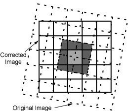
Geometric correction is transforming distorted remote sensing imagery into a spatially accurate format. This is achieved by adjusting the relationship between the image coordinate system (based on the sensor’s pixel layout) and the geographic coordinate system (often latitude/longitude or a map projection). The process requires calibration data, sensor position and attitude information, ground control points (GCPs), and other factors like atmospheric conditions.
Methods of Geometric Correction
1. Systematic Correction:
- Systematic correction is based on known and calibrated data. If the sensor’s geometry is well-defined (e.g., through camera calibration parameters), this method can remove distortions theoretically. For example, the collinearity equation (which describes the geometry between a sensor, image coordinates, and ground coordinates) is used for optical cameras. The equations are derived from sensor calibration, including parameters like lens distortion and fiducial marks.
- Example: In an optical camera, the geometry can be described by the collinearity equation, where the relationship between the image and ground coordinates is known through calibration data.
2. Non-Systematic Correction:
- Non-systematic correction is often used when exact sensor geometry isn’t available. This method uses polynomials to relate the geographic coordinates to the image coordinates through the known coordinates of Ground Control Points (GCPs). A least-squares method is typically used to solve the polynomial equations.
- The order of the polynomial (first-order, second-order, etc.) determines the degree of flexibility in the correction. Higher-order polynomials may fit the data more accurately but can also lead to overfitting if too many parameters are used.
- Accuracy is influenced by the number and distribution of GCPs. The more GCPs you have, the more reliable the transformation will be.
3. Combined Method:
The combined method first applies systematic correction and then uses polynomials to correct residual errors. This approach is often the most effective, as it addresses both the known and unknown distortions in the image. The goal is to achieve an error margin of about ±1 pixel in the final image.
Coordinate Transformation in Geometric Correction
Coordinate transformation plays a pivotal role in geometric correction. It converts the image coordinates into geographic coordinates using a set of known reference points (GCPs).
- Selection of Transformation Formula: Depending on the distortions, a suitable mathematical model is chosen. Common models include affine or polynomial transformations. For most remote sensing images (e.g., Landsat), a third-order polynomial is typically sufficient.
- Ground Control Points (GCPs): The quality and distribution of GCPs are critical. More GCPs result in better accuracy, but the GCPs should be well-distributed across the image, including at the corners and along edges. The least-squares method is used to adjust the parameters iteratively, minimizing the error.
Collinearity Equation
The collinearity equation is a physical model used to describe the geometry of optical remote sensing systems. It links the sensor position, the object on the ground, and the image coordinates.
- In this model, rays originating from the sensor’s projection centre intersect the ground at a specific point, which corresponds to the image coordinate. The collinearity equation describes this relationship and can be solved to obtain the ground coordinates from the image coordinates (and vice versa).
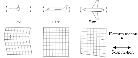
- For example, in optical mechanical scanners and CCD arrays, the cross-track direction often follows a central projection (similar to a frame camera), while the along-track direction is nearly parallel but slightly affected by sensor motion.
Resampling and Interpolation
Once the geometric transformation has been applied, the image is resampled to fit the new coordinate system. The process involves interpolation, where values are estimated for new pixel locations.
- Methods of Resampling:
- Nearest Neighbor (NN): The value of the closest pixel is assigned. This is fast but can introduce geometric errors of up to half a pixel.
- Bilinear Interpolation (BL): The pixel value is calculated based on the weighted average of the surrounding four pixels. This method produces smoother images but is more computationally expensive.
- Cubic Convolution (CC): The value is interpolated using a cubic function based on the 16 closest pixels. It results in smoother images with sharp details but requires more computation.
Map Projection
Finally, the image is projected onto a two-dimensional plane using a map projection. Since the Earth is a 3D ellipsoid, projecting it onto a flat surface always involves some distortion.
- Common Projection Types:
- Perspective Projection (e.g., Polar Stereo projection): Projects the Earth from a single point.
- Conical Projection (e.g., Lambert Conformal Conic): Projects the Earth onto a cone.
- Cylindrical Projection (e.g., Mercator, UTM): Projects the Earth onto a cylinder.
Universal Transverse Mercator (UTM) is widely used in remote sensing for large-scale mapping, as it minimises distortions for relatively small areas (about 6 degrees of longitude).
Accuracy of Geometric Correction
The accuracy of the geometric correction is typically measured in terms of the root mean square error (RMSE), which is calculated by comparing the corrected image coordinates to the known GCPs.
Accuracy Formula:
The standard deviation (in pixels) of the transformed coordinates from the reference coordinates can be calculated as: $$ u = \frac{1}{n} \sum_{i=1}^{n} |u_i – f(x_i, y_i)| \\ \text{where }\\ u_i \text{ and } v_i \text{ are the image coordinates of the GCP,}\\ \text{and } f(x_i, y_i) \text{ and } g(x_i, y_i) \text{ are the transformed coordinates based on the map reference system.}$$If the errors exceed the acceptable limit (usually ±1 pixel), the process may need to be revisited—either by adding more GCPs or adjusting the transformation method