The Frame of Varignon

The problem of finding the optimal location to set up an industry when more than one location of raw materials was available was found by French mathematician Pierre Varignon (1654-1722).

This problem uses the concept of the centre of mass, designed here in the form of a device known as the Frame of Varignon.

To understand this, let us first understand the concept of the centre of mass.

In Physics, the centre of mass of a distribution of mass in space or of a system of masses is a point (also known as a balance point) where the entire mass of the system is supposed to be concentrated or in simple words, the object balances itself at that point.

Mathematical treatment:
varignon-4ca7e72c-e88a-4ac7-825b-630935a325e3
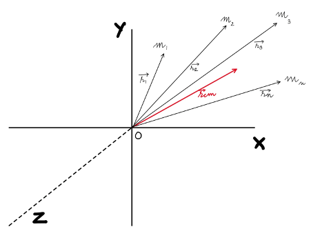
Consider a system of n n n n n objects distributed in space having masses m 1 , m 2 , m 3 … … … … … … m n m 1 , m 2 , m 3 … … … … … … m n m_(1),m_(2),m_(3)dots dots dots dots dots dotsm_(n) m_1, m_2, m_3 \ldots \ldots \ldots \ldots \ldots \ldots m_n m 1 , m 2 , m 3 … … … … … … m n respectively and their the centre of mass with respect to the origin of such a system is given by r c m → r c m → vec(r_(cm)) \overrightarrow{r_{c m}} r c m → and is defined by:
r c m → = m 1 r 1 → + m 2 r 2 → + m 3 r 3 → + ⋯ … … … … + m n r n → m 1 + m 2 + m 3 + ⋯ … … … … + m n r c m → = m 1 r 1 → + m 2 r 2 → + m 3 r 3 → + ⋯ … … … … + m n r n → m 1 + m 2 + m 3 + ⋯ … … … … + m n vec(r_(cm))=(m_(1) vec(r_(1))+m_(2) vec(r_(2))+m_(3) vec(r_(3))+cdots dots dots dots dots+m_(n) vec(r_(n)))/(m_(1)+m_(2)+m_(3)+cdots dots dots dots dots+m_(n)) \overrightarrow{r_{c m}}=\frac{m_1 \overrightarrow{r_1}+m_2 \overrightarrow{r_2}+m_3 \overrightarrow{r_3}+\cdots \ldots \ldots \ldots \ldots+m_n \overrightarrow{r_n}}{m_1+m_2+m_3+\cdots \ldots \ldots \ldots \ldots+m_n} r c m → = m 1 r 1 → + m 2 r 2 → + m 3 r 3 → + ⋯ … … … … + m n r n → m 1 + m 2 + m 3 + ⋯ … … … … + m n
Implementation in the Frame of Varignon:
The problem stated above is defined in a 2-D space, hence, to solve it the above stated definition can be reduced to two- dimensional vector space using only the x x x x x and y y y y y axes.
r c m x → = m 1 x 1 → + m 2 x 2 → + m 2 x 3 → + ⋯ + ⋯ ⋯ + … + m n x n → m 1 + m 2 + m 3 + ⋯ + ⋯ + ⋯ + m n r c m x → = m 1 x 1 → + m 2 x 2 → + m 2 x 3 → + ⋯ + ⋯ ⋯ + … + m n x n → m 1 + m 2 + m 3 + ⋯ + ⋯ + ⋯ + m n vec(r_(cm)x)=(m_(1) vec(x_(1))+m_(2) vec(x_(2))+m_(2) vec(x_(3))+cdots+cdots cdots+dots+m_(n) vec(x_(n)))/(m_(1)+m_(2)+m_(3)+cdots+cdots+cdots+m_(n)) \overrightarrow{r_{c m} x}=\frac{m_1 \overrightarrow{x_1}+m_2 \overrightarrow{x_2}+m_2 \overrightarrow{x_3}+\cdots+\cdots \cdots+\ldots+m_n \overrightarrow{x_n}}{m_1+m_2+m_3+\cdots+\cdots+\cdots+m_n} r c m x → = m 1 x 1 → + m 2 x 2 → + m 2 x 3 → + ⋯ + ⋯ ⋯ + … + m n x n → m 1 + m 2 + m 3 + ⋯ + ⋯ + ⋯ + m n
The implementation of the centre of mass system in the Frame of Varignon can be understood as: m n = m n = m_(n)= m_n= m n = The cost of transportation from n e h n e h n^(eh) n^{e h} n e h source to industry r c m → = r c m → = vec(r_(cm))= \overrightarrow{r_{c m}}= r c m → = The location of the industry
Now let us understand this problem with the help of an example:
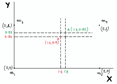
Consider 4 masses distributed in 2-D space as shown, with m 1 = 2 k g , m 2 = 4 k g , m 3 = 6 k g , m 4 = m 1 = 2 k g , m 2 = 4 k g , m 3 = 6 k g , m 4 = m_(1)=2kg,m_(2)=4kg,m_(3)=6kg,m_(4)= m_1=2 \mathrm{~kg}, m_2=4 \mathrm{~kg}, m_3=6 \mathrm{~kg}, m_4= m 1 = 2   k g , m 2 = 4   k g , m 3 = 6   k g , m 4 = 8kg. (The coordinates specify the position with respect to x x x x x and y y y y y axes)
varignon-2-b871bb3e-7ac2-4607-abb5-fbfaf54384ee
τ c m x → = m 1 x 1 → + m 2 x 2 → + m 3 x 3 → + ⋯ … … … … … + m n x n → m 1 + m 2 + m 3 + ⋯ … … … + m n = 200 + 402 + 6 ∗ 0 + 8 × 2 2 + 4 + 6 + 8 = 1.2 τ c m x → = m 1 x 1 → + m 2 x 2 → + m 3 x 3 → + ⋯ … … … … … + m n x n → m 1 + m 2 + m 3 + ⋯ … … … + m n = 200 + 402 + 6 ∗ 0 + 8 × 2 2 + 4 + 6 + 8 = 1.2 vec(tau_(cm)x)=(m_(1) vec(x_(1))+m_(2) vec(x_(2))+m_(3) vec(x_(3))+cdots dots dots dots dots dots+m_(n) vec(x_(n)))/(m_(1)+m_(2)+m_(3)+cdots dots dots dots+m_(n))=(200+402+6**0+8xx2)/(2+4+6+8)=1.2 \overrightarrow{\tau_{c m} x}=\frac{m_1 \overrightarrow{x_1}+m_2 \overrightarrow{x_2}+m_3 \overrightarrow{x_3}+\cdots \ldots \ldots \ldots \ldots \ldots+m_n \overrightarrow{x_n}}{m_1+m_2+m_3+\cdots \ldots \ldots \ldots+m_n}=\frac{200+402+6 * 0+8 \times 2}{2+4+6+8}=1.2 τ c m x → = m 1 x 1 → + m 2 x 2 → + m 3 x 3 → + ⋯ … … … … … + m n x n → m 1 + m 2 + m 3 + ⋯ … … … + m n = 200 + 402 + 6 ∗ 0 + 8 × 2 2 + 4 + 6 + 8 = 1.2
r c m Y → = m 1 y 1 → + m 2 21 → + m 3 3 → + ⋯ … … … … + m n n → m 1 + m 2 + m 3 + ⋯ … … … … + m n = 2 ∗ 0 + 4 ∗ 0 + 6 ∗ 1 + 8 ∗ 1 2 + 4 + 6 + 8 = 0.7 r c m Y → = m 1 y 1 → + m 2 21 → + m 3 3 → + ⋯ … … … … + m n n → m 1 + m 2 + m 3 + ⋯ … … … … + m n = 2 ∗ 0 + 4 ∗ 0 + 6 ∗ 1 + 8 ∗ 1 2 + 4 + 6 + 8 = 0.7 vec(r_(cmY))=(m_(1) vec(y_(1))+m_(2) vec(sqrt21)+m_(3) vec(sqrt3)+cdots dots dots dots dots+m_(n) vec(sqrtn))/(m_(1)+m_(2)+m_(3)+cdots dots dots dots dots+m_(n))=(2**0+4**0+6**1+8**1)/(2+4+6+8)=0.7 \overrightarrow{r_{c m Y}}=\frac{m_1 \overrightarrow{y_1}+m_2 \overrightarrow{\sqrt{21}}+m_3 \overrightarrow{\sqrt{3}}+\cdots \ldots \ldots \ldots \ldots+m_n \overrightarrow{\sqrt{n}}}{m_1+m_2+m_3+\cdots \ldots \ldots \ldots \ldots+m_n}=\frac{2 * 0+4 * 0+6 * 1+8 * 1}{2+4+6+8}=0.7 r c m Y → = m 1 y 1 → + m 2 21 → + m 3 3 → + ⋯ … … … … + m n n → m 1 + m 2 + m 3 + ⋯ … … … … + m n = 2 ∗ 0 + 4 ∗ 0 + 6 ∗ 1 + 8 ∗ 1 2 + 4 + 6 + 8 = 0.7
Hence, the industry must be located at point A A A A A (shown in figure) with coordinates ( 1.2 , 0.7 ) ( 1.2 , 0.7 ) (1.2,0.7) (1.2,0.7) ( 1.2 , 0.7 ) .
Now, let the mass m 4 m 4 m_(4) m_4 m 4 be increased to 12 k g 12 k g 12kg 12 \mathrm{~kg} 12   k g . Recalculating the position of centre of mass:
varignon-3-43665e3d-c5ef-476b-aac1-eca4b5be9260
r c m X → = m 1 x 1 → + m 2 x 2 → + m 3 x 3 → + ⋯ … … … … … … + m n x n → m 1 + m 2 + m 3 + ⋯ … … … … + m n = 2 ∗ 0 + 4 ∗ 2 + 6 ∗ 0 + 12 ∗ 2 2 + 4 + 6 + 12 = 1.3 r c m Y → = m 1 y 1 → + m 2 y 2 → + m 3 y 3 → + ⋯ … … … … … … + m n y n → m 1 + m 2 + m 3 + ⋯ … … … … + m n = 2 ∗ 0 + 4 ∗ 0 + 6 ∗ 1 + 12 ∗ 1 2 + 4 + 6 + 12 = 0.75 r c m X → = m 1 x 1 → + m 2 x 2 → + m 3 x 3 → + ⋯ … … … … … … + m n x n → m 1 + m 2 + m 3 + ⋯ … … … … + m n = 2 ∗ 0 + 4 ∗ 2 + 6 ∗ 0 + 12 ∗ 2 2 + 4 + 6 + 12 = 1.3 r c m Y → = m 1 y 1 → + m 2 y 2 → + m 3 y 3 → + ⋯ … … … … … … + m n y n → m 1 + m 2 + m 3 + ⋯ … … … … + m n = 2 ∗ 0 + 4 ∗ 0 + 6 ∗ 1 + 12 ∗ 1 2 + 4 + 6 + 12 = 0.75 {:[ vec(r_(cmX))=(m_(1) vec(x_(1))+m_(2) vec(x_(2))+m_(3) vec(x_(3))+cdots dots dots dots dots dots dots+m_(n) vec(x_(n)))/(m_(1)+m_(2)+m_(3)+cdots dots dots dots dots+m_(n))=(2**0+4**2+6**0+12**2)/(2+4+6+12)=1.3],[ vec(r_(cmY))=(m_(1) vec(y_(1))+m_(2) vec(y_(2))+m_(3) vec(y_(3))+cdots dots dots dots dots dots dots+m_(n) vec(y_(n)))/(m_(1)+m_(2)+m_(3)+cdots dots dots dots dots+m_(n))=(2**0+4**0+6**1+12**1)/(2+4+6+12)=0.75]:} \begin{aligned} &\overrightarrow{r_{c m X}}=\frac{m_1 \overrightarrow{x_1}+m_2 \overrightarrow{x_2}+m_3 \overrightarrow{x_3}+\cdots \ldots \ldots \ldots \ldots \ldots \ldots+m_n \overrightarrow{x_n}}{m_1+m_2+m_3+\cdots \ldots \ldots \ldots \ldots+m_n}=\frac{2 * 0+4 * 2+6 * 0+12 * 2}{2+4+6+12}=1.3 \\ &\overrightarrow{r_{c m Y}}=\frac{m_1 \overrightarrow{y_1}+m_2 \overrightarrow{y_2}+m_3 \overrightarrow{y_3}+\cdots \ldots \ldots \ldots \ldots \ldots \ldots+m_n \overrightarrow{y_n}}{m_1+m_2+m_3+\cdots \ldots \ldots \ldots \ldots+m_n}=\frac{2 * 0+4 * 0+6 * 1+12 * 1}{2+4+6+12}=0.75 \end{aligned} r c m X → = m 1 x 1 → + m 2 x 2 → + m 3 x 3 → + ⋯ … … … … … … + m n x n → m 1 + m 2 + m 3 + ⋯ … … … … + m n = 2 ∗ 0 + 4 ∗ 2 + 6 ∗ 0 + 12 ∗ 2 2 + 4 + 6 + 12 = 1.3 r c m Y → = m 1 y 1 → + m 2 y 2 → + m 3 y 3 → + ⋯ … … … … … … + m n y n → m 1 + m 2 + m 3 + ⋯ … … … … + m n = 2 ∗ 0 + 4 ∗ 0 + 6 ∗ 1 + 12 ∗ 1 2 + 4 + 6 + 12 = 0.75

Hence, the industry must now be located at point B (shown in the figure) with coordinates (1.3, 0.75).

Clearly, from this calculation, it can be deduced that if the cost of transportation between one of the source locations to the industry is increased, then the optimal location of the industry shifts towards that source.

error: Content is protected !!