Mollweide’s Projection

The Mollweide projection is an equal-area projection that represents the world in an elliptical shape. This means that areas on the map are proportional to their corresponding areas on the globe. This makes it particularly useful for displaying global data, such as population density, climate zones, or land use, where the preservation of area is essential.

Mollweide’s projection is often used in world maps to balance the distortion of shapes and sizes, providing an accurate visual comparison of different regions.

Key Features

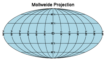
• Parallels of Latitude: The parallels are unequally spaced straight lines, but they are parallel to each other and the equator.
• Meridians of Longitude: The central meridian is a straight line, while all other meridians are equally spaced elliptical arcs that converge at the poles.
• Equal-Area Property: The projection is pseudocylindrical and equal-area, meaning it preserves the relative size of landmasses.
• Scale and Distortion: The scale is true only along the 40°44′ N and S parallels. Distortion is most severe near the outer edges and at high latitudes.
• Usage: It’s primarily used for global maps that display data distributions.

The Mathematics Behind Mollweide’s Projection

The Mollweide projection is a pseudocylindrical, equal-area map projection designed to display the entire globe on an elliptical surface. The parallels are unequally spaced straight lines, parallel to each other. The central meridian is a straight line, while all other meridians are equally spaced elliptical arcs that converge at the poles. The projection is based on a two-step mathematical process to convert geographic coordinates (latitude ϕ, longitude λ) into planar map coordinates (x,y). The first step involves finding an auxiliary angle (θ) by solving the transcendental equation:

2θ+sin(2θ)=πsinϕ

Once θ is known, the map coordinates are calculated using the formulas:

$$x=\frac{2\sqrt{2}}{\pi}R(\lambda-\lambda_0)\cos\theta$$

and

$$y = \sqrt{2}R\sin\theta$$

The resulting map is enclosed in an ellipse with a major axis four times the globe’s radius and a minor axis twice the globe’s radius. This mathematical process guarantees that the projection maintains the equal-area property.

It’s important to note that Karl Mollweide’s name is also associated with a set of unrelated trigonometric formulas, such as \(\frac{a+b}{c}=\frac{\cos\frac{\alpha-\beta}{2}}{\sin\frac{\gamma}{2}}\) and \(\frac{a-b}{c}=\frac{\sin\frac{\alpha-\beta}{2}}{\cos\frac{\gamma}{2}}\), which are used to check the solution of a triangle.

Example of Mollweide’s Projection

Question: Draw a graticule for Mollweide’s Projection showing the entire world on a scale of 1:250,000,000. The graticules should have 30° intervals for both latitudes and longitudes.

Solution:

To draw the Mollweide projection as shown in the image with a scale of 1:250,000,000, follow these step-by-step instructions:

Step 1: Set Up the Parameters

• Radius of the Earth (R): 6,371,000 meters or 6,371 km.
• Map Radius: The map scale is 1:250,000,000. So, convert the Earth’s radius to the map scale:
  \(R_{map} = \frac{6,371,000 \, \text{cm}}{250,000,000} = 2.5484 \, \text{cm}\)

Step 2: Draw the Elliptical Boundary

The Mollweide projection is an ellipse with a major axis (equator) twice the length of its minor axis (central meridian).

• Major Axis Length (the equator):$$4 \times R_{\text{map}} \times \sqrt{2}$$Calculation: 4×2.55 cm×1.414 ≈ 14.42 cm
• Minor Axis Length (the central meridian): $$2 \times R_{\text{map}} \times \sqrt{2}$$Calculation: 2×2.55 cm×1.414 ≈ 7.21 cm

Step 3: Mark the Parallels (Latitudes)

The parallels are straight, horizontal lines drawn at 30° intervals. Their distances from the central equator are calculated to maintain the equal-area property.

• Use the following formula to calculate the distance of each latitude from the centre (equator) on the map.
• The formula to use is \(y = \sqrt{2} \cdot R_{map} \cdot \sin(\theta)\) where \( \theta \) is the auxiliary angle derived from \(2\theta + \sin(2\theta) = \pi \sin(\phi)\)
• This gives us the approximate values for each latitude (in cm) from the centre:

Put the values into the formula and solve

\(y=\sqrt{2}(2.5484)\sin(0.8866)\)
\(y=(1.4142)(2.5484)(0.7744)\)
\(y\approx 2.793 \text{ cm}\)

Therefore, the y-coordinate for the 30° parallel is approximately 2.793 cm.

Latitude (ϕ)	sinϕ	Auxiliary Angle (θ in radians)	y-coordinate (cm)
90° N	1	1.5708	3.6044
60° N	0.866	1.4154	3.253
30° N	0.5	0.8866	2.2687
0°	0	0	0
30° S	-0.5	-0.8866	-2.2687
60° S	-0.866	-1.4154	-3.253
90° S	-1	-1.5708	-3.6044

• Measure the distances from the centre of your ellipse along the central meridian.
• Mark these points.
• Draw a straight, horizontal line through each of these marked points, extending it to the elliptical boundary.

Step 4: Mark the Meridians (Longitudes)

To draw the meridians for the Mollweide projection, you must plot a series of points and then connect them with a smooth, curved line. The meridians are elliptical arcs that converge at the poles. They are not equidistant across the map, but their spacing is uniform along the equator.

Let’s find the x-coordinate for the point at 30° North latitude and 60° East longitude.

The full formula to calculate the x-coordinate for a point on the Mollweide projection is: \(x = \frac{2\sqrt{2}}{\pi}R_{map}(\lambda – \lambda_0)\cos\theta\)

• Projected Radius (Rmap​): ≈2.5484 cm
• Longitude (λ): 60° E (which is π/3 radians)
• Central Meridian (λ0​): 0° (which is 0 radians)
• Auxiliary Angle (θ): ≈0.8866 radians (from the 30°N latitude calculation)

$$x=\frac{2\sqrt{2}}{\pi}(2.5484)\left(\frac{\pi}{3}\right)(0.6322)$$ x≈1.5204 cm

Therefore, the x-coordinate for the point at 30° North and 60° East is approximately 1.52 cm.

Latitude (ϕ)	y-coordinate (cm)	0°	30° E	60° E	90° E	120° E	150° E	180° E
90° N	3.6044	0	0	0	0	0	0	0
60° N	3.253	0	1.0504	2.1008	3.1512	4.2016	5.252	6.3024
30° N	2.2687	0	1.2023	2.4046	3.6069	4.8092	6.0115	7.2138
0°	0	0	1.2015	2.403	3.6045	4.806	6.0075	7.2088
30° S	-2.2687	0	1.2023	2.4046	3.6069	4.8092	6.0115	7.2138
60° S	-3.253	0	1.0504	2.1008	3.1512	4.2016	5.252	6.3024
90° S	-3.6044	0	0	0	0	0	0	0

• For each parallel you drew in Step 3, measure the distances from the central meridian using the table above.
• Mark a point for each longitude on each side of the central meridian.

Step 5: Draw the Graticules

• Draw the parallels (latitude lines) as horizontal lines spaced according to the distances calculated in Step 3.
• Draw the meridians (longitude lines) as curved lines that pass through the x-coordinates calculated in Step 4, ensuring they meet at the poles.